Jacob_Ray_Pehringer
Code Creation, The Way Nature Intended
July 24, 2025
After finishing my last project I felt a bit on edge. The last few years of the AI hype train has made me realize that we have a narrow window of time where we can still potentially contribute to the body of human knowledge. There will come a day in the not so distant future where humanity will no longer be in the driver’s seat, but merely a kid in a booster seat. Staring out the window of an ever accelerating car, trying to make sense of the i ncreasingly blurry shapes shooting by. So with this omnipresent feeling in my gut, I started searching for my next project . . .
Cellular Automata
I hopped on the hype train myself, but quickly found that I lacked both the math background and capital required to train even a small semi-cutting-edge model. So I shifted my focus to some sort of visualization project. The underlying matrix operations of older network architectures are simple enough to understand. I even managed to get some pretty solid results with NumPy and Matplotlib. But the whole idea felt a bit forced, I was working on the very thing that filled me with existential dread.
Then I rediscovered John Conway’s Game of Life after watching a recommended video of the game simulating itself, crazy! The game is simple, it takes place on a grid. Each grid cell can be either alive or dead. The state for each cell is determined by four rules:
1) Alive cells with less than two living neighbours die. 2) Alive cells with two or three living neighbours live. 3) Alive cells with more than three living neighbours die. 4) Dead cells with three living neighbours become alive.
 . # . .   . . . .   . . . .   . . . .   . . . .
 . . # .   # . # .   . . # .   . # . .   . . # .
 # # # .   . # # .   # . # .   . . # #   . . . #
 . . . .   . # . .   . # # .   . # # .   . # # #

  t = 0     t = 1     t = 2     t = 3     t = 4
glider pattern
With just these two states and four rules, the Game of Life is technically Turing-complete, meaning it could, in theory, compute anything given enough time and grid space!
This game falls within a broader model of computation called Cellular Automata (CA), which are basically zero-player games where grid cells follow basic rules based on their immediate neighbors. CA are awesome because they are easy to get into and offer many avenues of exploration. So I dusted off my mechanical pencil and grid paper to start creating my very own zero-player game!
Genetic Algorithms
I quickly discovered that building the rules for interesting behaviors was more difficult than I anticipated. I spent weeks trying different combinations of rules. Some of my attempts were quite complicated, involving cells with four or more possible states. It was fun and frustrating at the same time. It almost seemed random whether a set of rules was a dud or not.
Then one day it clicked, I bet a Genetic Algorithm (GA) could find an interesting set of rules. I first learned of GAs several years ago when I read about how NASA used one to find an optimal antenna design for one of their space probes. GAs are a class of optimization algorithms that closely mimic natural selection. They start out with a population of random solutions. Each solution is evaluated for how well it solves the problem at hand. The best solutions are chosen as parents, much like in nature. These parents combine their solutions to create new offspring solutions. Small mutations are then applied to the offspring. This evaluation, selection, reproduction, and mutation cycle repeats over and over, gradually evolving a population of solutions that are increasingly adept at solving the problem.
Evolving Project
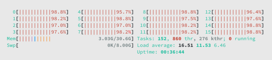
htop command
So I started creating a GA that could evolve CAs. But then I got to thinking, rules are basically just instructions right? If I’m already evolving instructions, why limit the scope to just CAs? What if I evolved small programs instead? This is when my project took off.
This launched me into four months of researching, developing, and testing a general purpose problem solving program. I am pretty happy with the results. Below is the contents of the projects README as of the posting of this write up. It’s short and sweet, describing what it is, and how to use it.
While I’m not an expert in the field of Linear Genetic Programming (LGP) the README also documents what I think are the novel approaches I took in the project (maybe they’re not novel and I’m just illiterate).
github.com/pehringer/finches/README.md
  //>
 //)    f  i  n  c  h  e  s
/ ^
Finches uses linear genetic programming (LGP) to evolve functions from input-output examples. The name finches comes from Darwin’s finches, the canonical example of the Theory of Evolution.
Use Cases
- Reverse Engineering - Infer hidden logic from observed inputs and outputs, even when source code or hardware is unavailable.
- Data Compression - Evolve compact functions that approximate large datasets, allowing for significant reductions in storage.
Use Finches
Run the Makefile to build finches:
$ make
go build -o finches
Create a examples.csv file where each line contains example input(s) followed by the SINGLE expected output.
A examples.csv file for a three input function:
2.175702178,3.4978843946,2.8679357454,42.7201735336
3.727866762,4.6107086188,-3.4225095225,70.7890623513
-1.6914281809,-4.2087394179,2.475850641,39.3184982846
0.4793454968,3.6758416723,-2.3773138762,24.9995146063
2.0264537683,-0.8547617596,-4.7856914722,68.217804457
-3.1671669278,-0.8226972678,-3.4907083169,49.9335397455
0.5837987947,-4.7796641015,-4.1819232422,51.3009229327
-3.8194496568,-0.2562750524,4.7254929564,77.767960022
-3.2942570245,2.4734392713,1.5534051521,-0.7628296637
-0.2975551098,-4.5018374909,0.5470816154,8.8745394888
0.8429004267,2.4176065495,-2.1438009046,22.0203497133
-0.8824430962,0.9755978955,0.7106055863,5.6755047387
-2.0692284587,-1.6842422241,-2.8357669579,38.1641150601
0.557997777,-4.339746829,-0.99579524,2.5736885366
4.4987170938,2.2281464346,4.1271759253,71.6496271677
3.9986431397,1.2608830478,-0.2652827417,11.2961243578
The above file contains 16 input-output examples, ideally you want at least 256 examples.
Run finches on examples.csv, adjust the –generations and or –individuals counts if the resulting error or number of instructions is too high:
$ ./finches examples.csv
instructions: 1 error: 69.621665% -> function.go
$ ./finches examples.csv --generations 4096
instructions: 47 error: 6.069102% -> function.go
$ ./finches examples.csv --generations 4096 --individuals 1024
instructions: 20 error: 0.000000% -> function.go
Genetic algorithms at their core rely on randomness so your result may vary.
Finches will evolve a function to fit the input-output examples and create a function.go file with equivalent Go code.
Executing function.go with the first example from input.csv:
go run function.go 2.175702178 3.4978843946 2.8679357454
42.720173532676014
The filepath for the evolved function can also be changed:
$ ./finches examples.csv --destination fooBar.go
instructions: 29 error: 7.706219% -> fooBar.go
Finches Instruction Set Architecture (ISA)
Finches ISA is specifically designed to optimize LGP evolvability, creating a smoother solution landscape for programs. Traditional LGP often rely on branching control flow operations, which easily break under genetic crossover and mutation, leading to a rougher fitness landscape. Finches, however, employs branchless programming techniques for its control flow. This approach integrates control flow directly into computations. By avoiding explicit branching, LGP can incrementally evolve conditional flow logic through symbolic regression, resulting in a significantly smoother solution landscape.
Furthermore, this ISA only contains arithmetic comparison operations (such as min, max, <, and >). This design choice provides a more incremental and continuous path for forming control flow logic when compared to all-or-nothing boolean operations (like AND, OR, NOT), further contributing to a smoother solution landscape.
Finally, the inclusion of inverse operations (e.g., addition and subtraction, multiplication and division, sine and arcsine) creates a more uniform and balanced search space. This allows instructions to be effectively “undone” or counteracted, which further contributes to a smoother solution landscape and enhances finches ability to explore.
These design choices, including the compact uniform 16-bit instruction format (where all bit combinations map to valid instructions), collectively contribute to a significantly reduced search space for LGP to explore. By constraining these architectural dimensions, finches can more efficiently navigate the solution landscape, making the evolutionary process faster.
Instruction Format:
| OPCODE | RESULT | FIRST | SECOND |
|---|---|---|---|
| [15-12] | [11-8] | [7-4] | [3-0] |
Instruction Set:
NOTE: Instructions return NaN (Not a Number) or Inf (Infinity) for invalid operands. This allows for continued program execution instead of program termination.
NOTE: Constants are preloaded into the registers before program execution. This eliminates the need for special registers and allows for uniform register access.
| OPCODE | Mnemonic | Pseudocode |
|---|---|---|
| 0000 | AD | register[RESULT] = register[FIRST] + register[SECOND] |
| 0001 | SB | register[RESULT] = register[FIRST] - register[SECOND] |
| 0010 | ML | register[RESULT] = register[FIRST] * register[SECOND] |
| 0011 | DV | register[RESULT] = register[FIRST] / register[SECOND] |
| 0100 | PW | register[RESULT] = pow(register[FIRST], register[SECOND]) |
| 0101 | SQ | register[RESULT] = sqrt(register[FIRST]) |
| 0110 | EX | register[RESULT] = exp(register[FIRST]) |
| 0111 | LG | register[RESULT] = log(register[FIRST]) |
| 1000 | SN | register[RESULT] = sin(register[FIRST]) |
| 1001 | AS | register[RESULT] = asin(register[FIRST]) |
| 1010 | CS | register[RESULT] = cos(register[FIRST]) |
| 1011 | AC | register[RESULT] = acos(register[FIRST]) |
| 1100 | MN | register[RESULT] = min(register[FIRST], register[SECOND]) |
| 1101 | MX | register[RESULT] = max(register[FIRST], register[SECOND]) |
| 1110 | LT | register[RESULT] = 1 if register[FIRST] < register[SECOND] else 0 |
| 1111 | GT | register[RESULT] = 1 if register[FIRST] > register[SECOND] else 0 |
Finches Genetic Algorithm (GA)
Finches GA is designed to be as simple as possible, yet still capable of eliciting complex and desirable evolutionary behaviors. It promotes slow population convergence, encourages depth-first and breadth-first exploration of the solution space, and manages genome size and bloat. Furthermore, it minimizes program breakage, ensuring genetic operations are less disruptive to evolving programs. All of these design choices not only contribute to a smoother fitness landscape but also directly enhance performance by simplifying computational overhead.
The major difference in the GA is the replacement of the traditional crossover operator with the Fission and Transfer operators. These two operators simulate horizontal gene transfer resulting minimal breakage and strong global exploration.
Additionally, the selection and replacement operators are designed to slow down premature convergence and enable robust local exploration. While their simplicity allows for fast execution and reduced memory allocations.
Algorithm:
- Initialization: Create a population of individuals. Each individual contains a very low fitness score, multiple (sixteen) random constants, and a single random instruction.
- Loop:
- Selection: Two neighboring parents are randomly selected from the population. A separate donor individual is also randomly selected from the population.
- Replacement: The parent with the lower fitness score (or if equal, the one with a higher instruction count) is selected to be the new offspring.
- Fission: The offspring’s instructions and constants are replaced with a copy of the remaining parent’s instructions and constants.
- Mutation: The offspring then undergoes one of the following mutations:
- A constant is randomly adjusted slightly.
- An instruction is randomly replaced (with a new random one).
- An instruction is randomly deleted.
- An instruction is randomly inserted (with a new random one).
- Transfer: With a small probability, a small random block of instructions from the donor is copied and randomly inserted into the offspring.
- Evaluation: The offspring’s fitness score is calculated by running a series of test cases. NaN or Infinity results are heavily penalized.
- Termination: The constants and instructions from the individual with the highest fitness score are returned.